Extended Description
Contaminants
ABICAM's mass-balance methodology is broadly applicable to a variety of indoor contaminants. A "contaminant" can be a chemical compound with a unique identifier, a specific strain of pathogen, or a collection of particles within a designated size range (e.g., < 2.5 microns).
ABICAM was originally designed to simulate semi-volatile organic compounds (SVOCs) in the gas-phase and various condensed phases, including particles. ABICAM was later expanded to include pathogens, such as severe acute respiratory syndrome coronavirus 2 (SARS-CoV-2), the virus responsible for the COVID-19 pandemic. For more information about specific applications of ABICAM, see Publications.
Indoor Microenvironments
An indoor microenvironment is a network of compartments (e.g., indoor air, surfaces, etc.) connected by contaminant mass-transfer rates. Examples of indoor microenvironments include a home, a workplace, and a vehicle. At any given time in a simulation, a microenvironment includes a base set of environmental compartments plus zero or more human occupants.
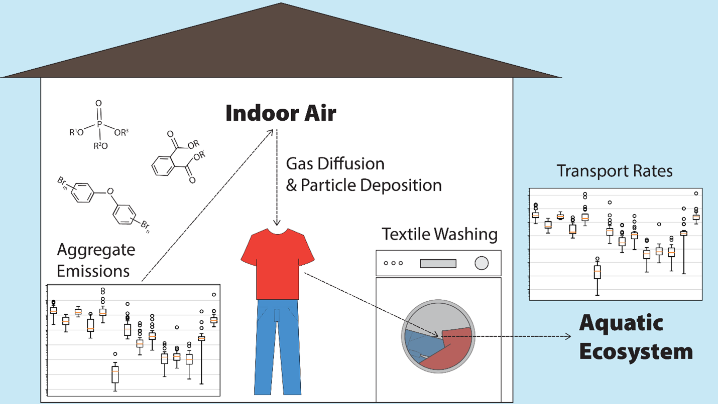
Figure 1. Example residential indoor microenvironment with associated chemical transport and removal processes.
Human Occupants
Like indoor microenvironments, human occupants also consist of compartments (e.g., clothing), which are coupled with those of the microenvironment in which they reside at a given time. Moreover, an occupant can move between indoor microenvironments and perform specific time-dependent activities within them.
Mass-Balance Models
Each indoor microenvironment is associated with one mass-balance model per simulated contaminant. The dynamics of a given contaminant are represented by a system of coupled, first-order, ordinary, linear, inhomogeneous differential equations with time-dependent coefficients. For a given mass-balance model associated with microenvironment e and contaminant c,
| \[\frac{d\vec{m}_e^c(t)}{dt} = \mathrm{K}_e^c(t) ~ \vec{m}_e^c(t) + \vec{E}_e^c(t)\] | (1) |
where \(\vec{m}_e^c(t)\) is a time-dependent vector of the mass of contaminant; \(\mathrm{K}_e^c(t)\) is a square matrix (possibly sparse) of order \(n\) containing time-dependent mass-transfer and removal rate coefficients \([\mathrm{T^{-1}}]\), where \(n\) is the number of compartments. Diagonal elements of \(\mathrm{K}_e^c(t)\) represent the sums of intercompartmental mass transfers and removals from the indoor system (e.g., through viral inactivation). Off-diagonal elements represent intercompartmental mass transfers (e.g., resuspension from clothing to air). \(\vec{E}_e^c(t)\) is a vector of contaminant emission rates or source terms \([\mathrm{M\cdot T^{-1}}]\), which can also be time-dependent (e.g., exhalation of pathogens to air). The time dependences of \(\mathrm{K}_e^c(t)\) and \(\vec{E}_e^c(t)\) arise from the influence of human activities.
Human Activities
A given human occupant's activities govern the mass-balance model(s) associated with the microenvironment in which they reside at a given time. Specifically, these activities determine the values of rate coefficients in the mass-balance equations (eqn 1), and thereby influence rates of contaminant mass transfer and removal. The values of these rate coefficients follow a piecewise-constant relationship with time, as shown in Figure 2.
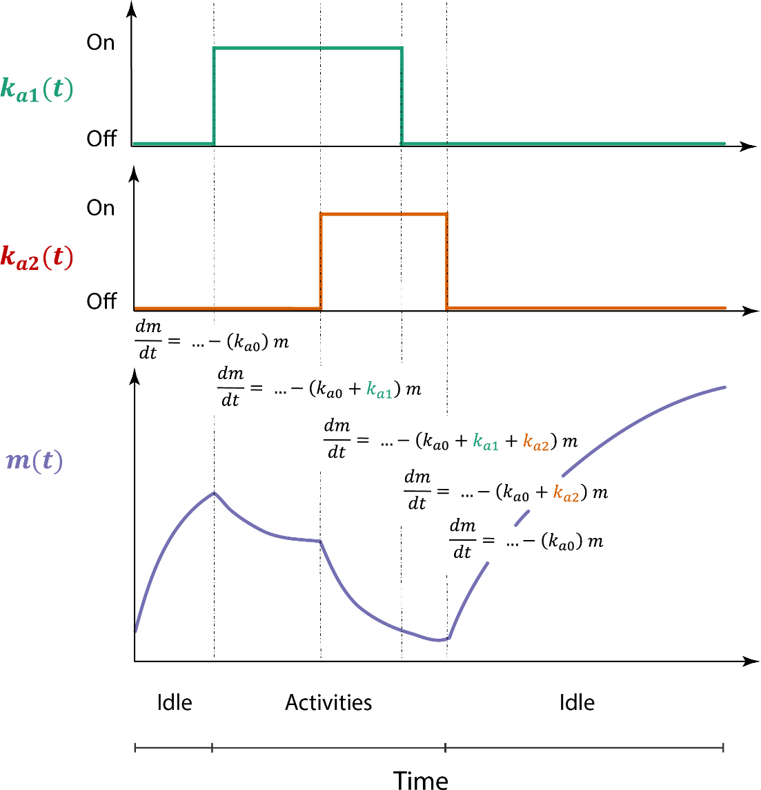
Figure 2. Overview of ABICAM's treatment of time-dependent parameters. Here, \(k_{a0}\) corresponds to a baseline removal rate coefficient \([\mathrm{T^{-1}}]\) for an arbitrary compartment, while \(k_{a1}\) and \(k_{a2}\) are time-dependent removal rate coefficients for two arbitrary activities (a1, a2). These latter two parameters are portrayed as being disabled or enabled as a function of time, depending on which activities are occurring. The total removal rate at time \(t\) governs the dynamics of contaminant mass, expressed as \(m(t)\), in this compartment.
Activity Schedules
An activity schedule maps a given human occupant's activities to specific time periods. Accordingly, this schedule determines which microenvironment they should reside in, and which activity to perform throughout each period. ABICAM combines the individual schedules of all occupants into a master schedule, which governs an exposure simulation. This collection is disjoint (non-overlapping) and thereby accounts for every change in activity that must occur at the desired time resolution (e.g., minutes or seconds). The individual schedules of occupants can be independent or correlated with respect to time. Accounting for correlated activities enables occupants to interact with each other. Such interactions can include (a) performing the same activity, (b) changing their location/microenvironment simultaneously, (c) residing in the same microenvironment, and (d) cross-contaminating each other through contaminant mass exchange.
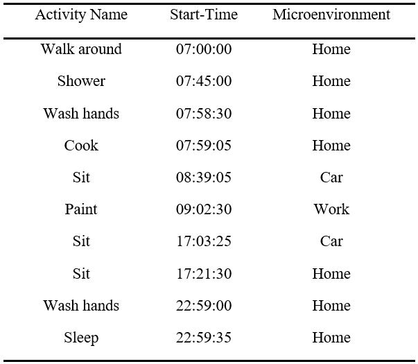
Figure 3. Example human activity schedule for one occupant. Activities are defined by a name and start-time (hour:minute:second).
Spatial Variability
In real indoor environments, contaminant concentrations in various media are rarely uniform. There are two ways in which ABICAM can account for spatial variability of contaminant concentrations: (1) near-field/far-field approach, and (2) finite volume method.
(1) A near-field/far-field approach is used to account for incomplete air mixing during static periods with relatively buoyant airflow. If at least one human occupant is present in a given microenvironment during a given period, ABICAM discretizes the indoor air compartment into a "far field" plus one "near field" for each occupant. The "near field" represents a convective boundary layer of air adjacent to a given occupant, which is coupled with the surrounding "far field" by an interzonal air exchange rate. One unique feature of ABICAM is its treatment of this interzonal air exchange rate as a dynamic parameter to account for time-dependent factors that influence airflow, such as human movement.
The near field couples a given human occupant and their compartments with the indoor microenvironment in which they resided during a given period. If an occupant moves from one microenvironment to another, each respective microenvironment's network of compartments, and thus \(\mathrm{K}_e^c(t)\) in eqn 1, is updated as illustrated in Figure 4.
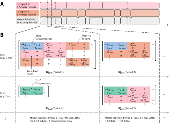
Figure 4. Overview of ABICAM's time-dependent matrices of rate coefficients for indoor microenvironments. (A) A "master schedule" maps the activities of two arbitrary human occupants (H1 and H2) to specific periods. To illustrate, each activity period is represented by a superellipse with length directly proportional to duration. (B) For a given contaminant (c), each indoor microenvironment is associated with a matrix [\(\mathrm{K}_e^c(t)\) in eqn 1]. The size of each matrix reflects the total number of compartments in the microenvironment and therefore changes as human occupants enter and leave. In this example, H1 moves from Env1 to Env2 as time progresses from Period 1 to Period 2, while H2 remains in Env1. Rate coefficients \([\mathrm{T^{-1}}]\) for contaminant mass transfer (\(\rightarrow\)) and removal (rem) are denoted by \(k\) with subscripts, nf, ff, x, and y referring to near field, far field, and arbitrary environmental and human compartments, respectively.
(2) For SVOCs, ABICAM uses a finite volume method to account for possible nonlinear chemical concentration profiles in non-air compartments due to molecular diffusion. This method discretizes the spatial dimension within the model's domain by representing each compartment as one or more finite volumes (or layers). This discretization translates the continuous diffusion problem, arising from Fick's laws, into a system of ordinary differential equations (eqn 1), which can be solved numerically for the spatial average mass of a given compound in each volume across time.
Data Inputs
The input parameters of ABICAM can be divided into two general categories: (a) physical parameters for constructing mass-balance model(s) for each microenvironment and contaminant (eqn 1); (b) activity parameters for generating an activity schedule for each human occupant (e.g., Figure 3). These parameters either be user-defined, or generated probabilistically at run-time through Monte Carlo simulation to account for interindividual variability and parameter uncertainty. A configuration file (JSON) specifies which indoor microenvironments and human occupants to include in a simulation, file paths to associated input data, and other simulation details.
Simulations
After loading the input data, initializing the indoor microenvironment(s) and human occupant(s), and constructing the mass-balance model(s), a simulation can be run generally as follows:
For each period in the master schedule:
- (1) Pass the time state information to each human occupant.
- (2) Occupants relocate to the correct indoor microenvironments(s) as needed.
- (3) Occupant activities are initialized as needed.
- (4) Mass-balance models are updated according to (2) and (3).
- (5) For each indoor microenvironment:
- (b) Compute the dynamics for each mass-balance model by solving the initial value problem numerically (eqn 1).
- (a) Store the resulting time series separately for each microenvironment and occupant and their respective compartments.
Exposure Histories
Throughout a simulation, each human compartment develops an "exposure history" for each contaminant (e.g., number of viable SARS-CoV-2 virions on clothing). This history represents the dynamics of contaminant exposure across all activity periods in the master schedule. By retaining their exposure histories, occupants can also function as vectors for transporting contaminants across indoor microenvironments, while subsequently exposing themselves and any bystanders.
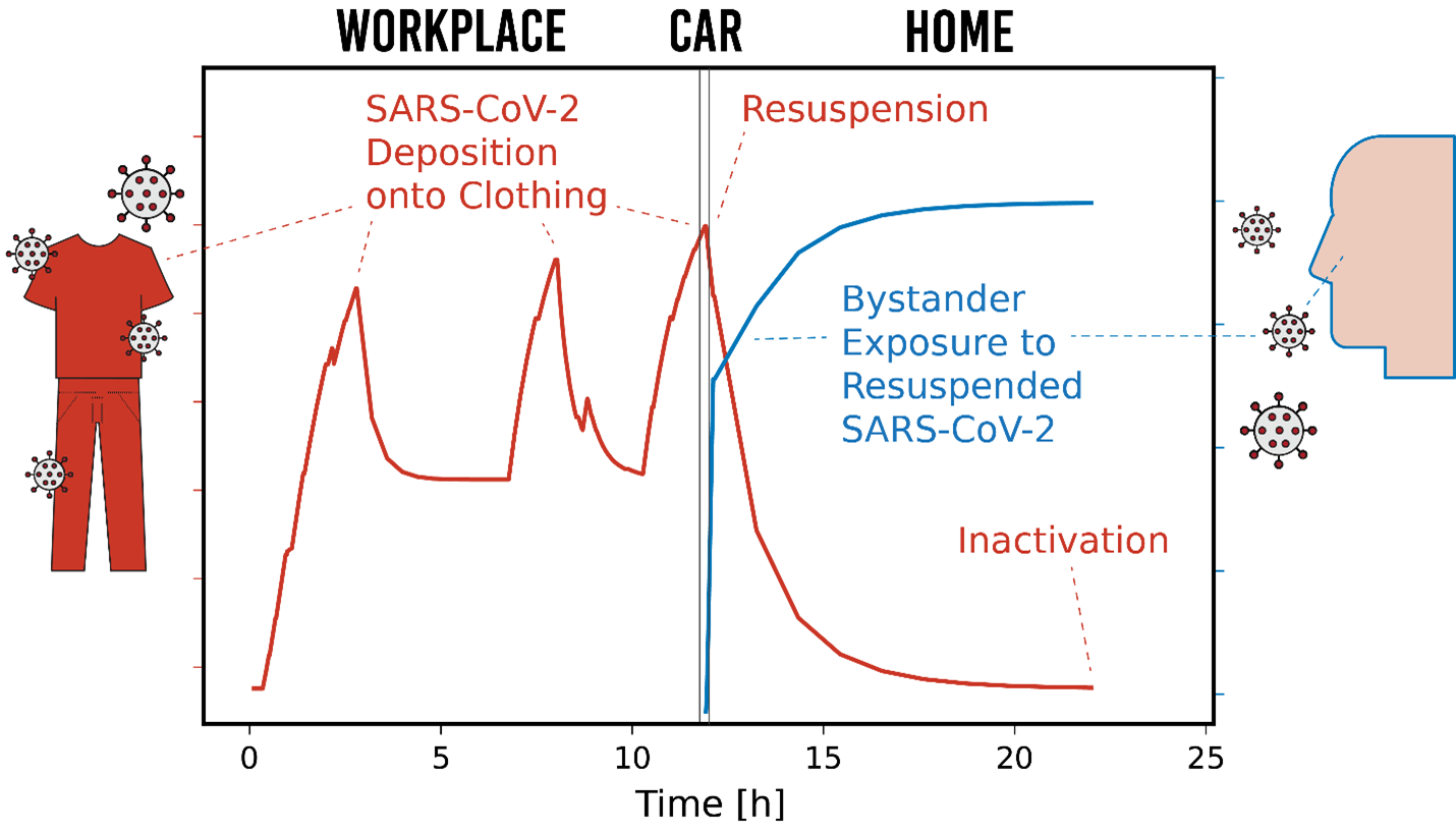
Figure 5. Example exposure histories of SARS-CoV-2 on clothing and corresponding cumulative inhalation exposure of a bystander.